Guest Posts – Page 16 – The OM Blog by Heizer, Render, & Munson

Guest Post: Operations Management on Vacation

Our Guest Post today comes from Prof. Howard Weiss, at Temple University. Howard is the developer of the POM for Windows and Excel OM problem solving software that we provide free with our OM texts.

I went on vacation last week to Florida. I enjoyed seeing Barry in Orlando for dinner and loved taking my grandson to the theme parks. But as an Operations Management professor, I can’t help but to be alert to possible system improvements.

Layout: I stayed at a hotel that had a buffet breakfast that was arranged in a straight line. The first process was a milk dispenser followed by the cereal followed by the bowls. You do not need to be an operations expert to realize that this will cause problems. And it did!

Aggregate Planning: The hotel’s breakfast capacity was based on a normal day where demand was spread out from 6:30-9:30. However, on this rainy day, guests were in no rush to visit the amusement parks and there was a large demand for breakfast from 9:00-9:30. The hotel could have prepared more food in the previous production period of 8:30-9:00 and held it until 9:00 to lessen the backlog.

Reliability: At another hotel the extension cord that was used for the waffle irons became defective. The kitchen had no backup extension cord.

Process Design: At the Miami Airport the moving walkways have signs that say “Stand on right, walk on left.” This made the process much more efficient than other moving walkways or the DC Metro that do not have the signage. For an interesting read see http://www.welovedc.com/2010/07/20/dc-mythbusting-stand-to-the-right/

Operating Costs: We saw an escalator that was not functioning. This reminded me that many escalators in Europe run only when someone approaches them. This saves energy. If an escalator is not running in the US it is because it is broken.

Safety: When we exited the plane we saw that a passenger who had been sitting in the emergency row, now on a wheelchair by the plane’s exit, waiting to be wheeled away. You would think that the airline’s information system would flag a passenger who needs a wheelchair from sitting in the exit row.

Guest Post: Beat the Instructor–A Great Classroom Forecasting Exercise

Our Guest Post today comes from Brent Snider, who is an award winning instructor of Operations Management at the University of Calgary’s Haskayne School of Business.

Forecasting is covered late in the term in our required undergrad course, which may contribute to student apathy towards the topic. Beat the Instructor was developed after recognizing that there were no spreadsheet-based experiential introductory exercises that have been shown to build significant student interest in learning forecasting techniques.

Most forecasting exercises tend to be highly technical and or intended to be used after forecasting techniques have already been introduced in lectures. Beat the Instructor is an in-class game that enables student groups to compete against their instructor in an introductory time-series forecasting exercise, even before any lecture content has been covered. In addition to starting the forecasting topic positively via a 30 minute hands-on experiential learning exercise, the game has proven to build strong student interest in learning the forecasting techniques that are covered later in the lecture.

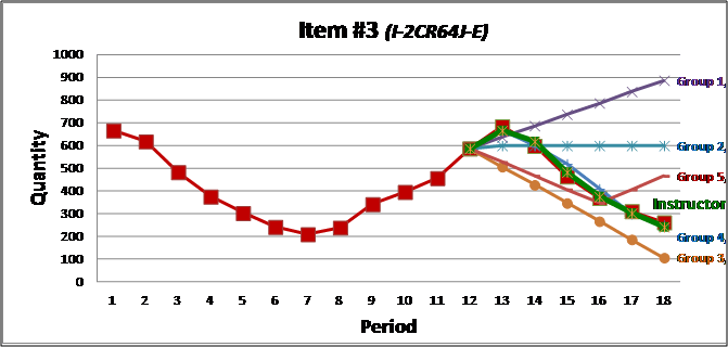
Student groups are provided a spreadsheet with historical demand for 12 previous periods for 4 separate items. Each of the 4 items represents one of the classical demand patterns of trend, cycles, seasonality, and random variations. The students are then asked to predict demand for the next 6 periods for each item, and submit their forecast to the instructor. In addition to competing amongst themselves, student groups are challenged to outperform the instructor’s forecast (who also predicts demand using the techniques that will be subsequently covered). Each group’s forecast is graphed, in addition to the instructor’s, creating anticipation for the actual demand pattern. After actual demand is randomly generated (and revealed on the graph), each group’s forecast error is calculated and ranked. Typically the instructor outperforms most if not all groups, generating student interest in learning the techniques that can answer their often posed question: “How did you forecast so well?”

Guest Post: How Much Inventory is There in the World?

Today’s Guest Post comes from Kelly Thomas, who is a supply chain management professional and executive at JDA Software.

Here is a simple question: “how much inventory is in the world?” The short answer is that no one knows for sure, and no one keeps track of it at a global level. It’s an interesting question though, because it gives us an understanding of how efficient the world is in turning inventory into economic output.

The Council of Supply Chain Management Professional’s annual report leverages data from the Bureau of Economic Affairs and other sources, and provides great detail on logistics, distribution, and inventory costs in the U.S. According to this report, there was $2.2 trillion in business inventory in the U.S. in 2012. Also last year, there was about $70T worth of economic output globally. The U.S. represented approximately 22% of overall output. Assuming the rest of the world is as efficient as the U.S., a simple pro-rata calculation based on economic output produces a global inventory level of $2.2T/22% = $10T.

This calculation does not account for the relative efficiency of economic activity across countries. China, for example, has twice the logistics costs of the U.S. as a percentage of economic activity or GDP. Given that the combined GDP of the BRIC countries is almost the size of the U.S. economy, and if you assume all of the BRIC countries have logistics costs similar to that of China, this would add almost another $2T to the overall inventory number, yielding $12T in global inventory. This likely understates the actual number since it also does not account for relative inefficiencies in other emerging markets (and does not include government-owned inventories).

This ballpark estimate gives us an understanding of the efficiency of economic output relative to inventory. Based on this information, economic output turns against inventory are about 6 (roughly the same as sales turns). This means there is approximately 2 months of global inventory sitting around at any one time (on an economic output basis). We can do better than 6 turns. If we were able to reduce inventories by just 10%, that would free up $1.2T in capital that could be deployed to growth activities that would benefit companies, countries, and ultimately people.

Guest Post: Using MyOMLab at San Francisco State University

Dr. Ozgur Ozluk is Associate Professor of Decision Sciences at San Francisco State University. Click here to see his syllabus, which is posted on our blog.

When I heard of MyOMLab, developed for our Heizer-Render textbook, a few years ago, I nearly jumped out of my seat. If you are teaching at a state university with no Ph.D. program (read no Teaching Assistants), it seems impossible to stay afloat over the sea of grading during a semester. Exams, homework assignments, projects, quizzes keep piling up.

So I immediately signed up for MyOMLab. After a bit of a learning curve, it was a breeze to set up online homework assignments/quizzes for my classes. At the start, there were some painful moments, requisite with any technological adoption. But the members of support group for MyOMLab were responsive, helpful and open to constructive feedback. Once the few kinks were cleared, this online platform became an integral component of my teaching. I definitely felt less over-worked and more relaxed.

And what about the students? I can safely report that they are also satisfied with the experience. The beginning of every semester is not without its trials and tribulations, while the students are trying to feel their way through the online system. However, within a few weeks they feel at ease with using MyOMLab. They are happy to they have an assessment tool that provides them almost instantaneous feedback and helps them with their meta-cognition skills. Pairing the online platform with my office hours makes it a great learning experience. It is a win-win situation for both the teacher and the student.

In a recent conversation with Jay and Barry at the San Antonio INFORMS meeting, I was shocked to hear that only a quarter of the instructors who use their OM textbook utilize this robust and versatile online assessment platform. If you are of this three-quarters majority and still reading, you owe it to yourself to give MyOMLab a try. You will not regret it!

“

Guest Post: A Teaching Tip for Visualizing Waiting Line Flows and Interarrival Times

While Jay and Barry attend the INFORMS meeting in San Antonio, Dr. Steven Harrod, Assistant Professor of Operations Management at the University of Dayton provides this, his 5th Guest Post for our blog.

I find in teaching Waiting Line Models in Module D of the Heizer/Render text that the definitions and relationship of rates of flow and inter-arrival times are frustratingly difficult for some students to grasp. Here is a classroom exercise that may help:

Introduce the following video (http://youtu.be/O84FlZnP0qs ), explaining that it shows traffic starting after a red light turns to green. Start the video at 0:17 (prepare the video in advance so you don’t have to watch the commercial during lecture). Draw the students’ attention to the second lane of traffic, headed by the Range Rover.

Explain that this flow of traffic may be described either by how many cars cross the white stop line in a period of time, or by how long each car takes to cross the line. Either way, the traffic flow described is identical. Play the video, and count ten cars across the line (ignore the car that changes lanes). Car number ten is a yellow cab, so stop the video with the eleventh car at the white line. You should find the video counter at 0:42, or 25 elapsed seconds. This is a flow of 10 cars in 25 seconds, or 10/25 cars per second, or 1440 cars per hour.

Restart the video at 0:17. Now, count the seconds between each successive car at the white line. They are, approximately, 5, 3, 2, 1, 3, 2, 2, 3, 2, and 2. The average time between cars is then 2.5 seconds. Now, since in both cases we have witnessed the same traffic flow, make the argument that these two measurements are equivalent. Indeed they are, after you explain that the inter-arrival time of a flow and the rate of flow are inverses of each other. In this case in particular, (1/2.5) = (10/25) and [1/(10/25)] = 2.5.

For some students, this is a difficult concept, and I repeat this approach multiple times in the course.

Guest Post: Approaches for Engaging OM Students in a Study Abroad Class

Our Guest Post (his 8th) comes from Phillip Flamm, who teaches OM in the ISQS Department at Texas Tech University.

I have been selected to teach operations management this summer in the Texas Tech University Rawls College of Business Study Abroad Program in Spain. After recovering from the initial shock of logistical planning I began to think about what it would take to keep fifteen 20 year olds engaged for a month while they are facing the distraction of “things to do in a foreign country.” It occurred to me that the key to making this work is “keeping the students consistently engaged.” I came up with several ideas that might help to keep the students awake and productive in a small class setting:

Divide the students into teams of 3
Each member of the team will get the same final grade for 80% of the class so they will be forced to help each other
Grades will be based on 2 exams (taken as a team), 2 or 3 team presentations, and a peer grade (from team members plus an attitude grade from me)
One presentation will be a tutorial of quantitative material (basically teaching the class quantitative material)
The second presentation will be the team solution of an operations management case scenario

This seems to be an opportunity to create an atmosphere very nearly like the day-to-day business world. Every day workers create designs, solve problems, make decisions, prepare presentations, and receive rewards as teams. I am curious to see how the students will respond to dealing with problems that teams normally encounter when their grade depends upon how they handle themselves. The first day of class I will cover interpersonal skills topics to include conflict resolution and team building. Upon completion of this program I will enter an “after Spain” blog covering results. As part of the class, I have also arranged tours of 2 manufacturing plants.

Guest Post: Another Approach to Teaching the Center-of-Gravity Model

Your Heizer/Render textbook covers the Center-of-Gravity Method in Chapter 8. However, there is a related model that is not covered and is easy to explain to the students. Consider Example 3 in the text, on page 322, in which Quain’s Discount Department Stores is looking for a location to build a new warehouse. Suppose though that rather than seeking a “central” location, the warehouse must be built in one of the four cities that currently has a store – Chicago, Pittsburgh, New York or Atlanta.

This revised example can lead to the discussion of straight-line (Euclidean) distance as compared with city-block/taxi distance and can serve as a student reminder about the Pythagorean Theorem. The distance computations are tedious but not difficult. Of course, using POM for Windows (shown below)

or Excel OM (below) the students can easily identify that Pittsburgh is the city with the least total weighted movement from each of the other 3 cities with a total weighted movement of 318,692.

Guest Post: Making LP Relevant to Students

Dr. Steven Harrod is Assistant Professor of Operations Management at the University of Dayton. He shares a tip on teaching LP today.

It takes some creativity to make linear programming (see Module B in the Heizer/Render text) relevant to students. Here is an activity that offers a discussion of energy, transportation, and air pollution. The topic is coal-burning electric power plants, and it is an example of the blending problem.

Nearly half of all electricity in the U.S. is produced by burning coal, and nearly all of this coal moves by rail. Coal is an organic material that varies considerably in cost, power, and pollution content. Power plants frequently blend different coals to achieve their desired performance. Trains magazine published a detailed article on the movement of coal and its consumption by electric power plants in 2010. The readings and class materials may be downloaded here.

The documents package includes a quiz you may assign to motivate the reading assignment, a longer version of this Guest Post, and a sample spreadsheet model. Start the class discussion by drawing the class’s attention to the power plant at Monroe, Michigan. If you have an overhead projector with internet access, use Google maps to display a satellite photo of the plant. The lakeside plant has a prominent railroad loop and coal storage facility. You may also wish to explain how a power plant converts coal into electricity, and the environment concerns (sulfur causes acid rain and ash must be disposed of).

The challenge question for the students is: what coal should this plant purchase to satisfy energy and pollution limits at minimum cost? The formulated and solved LP leads to an optimal blend of three of the five coal sources. Ask the students, “is this intuitive?” Would you have been able to reach this conclusion without LP? Discuss at length and experiment with reducing or eliminating the pollution limits. This exercise may lead to a lengthy discussion of energy policy, environmental policy, and their joint effect on transportation demand.

Guest Post: Tying Scheduling Back to Operations Strategy in Your Course

Dr. Steven Harrod is Assistant Professor of Operations Management at the University of Dayton and can be reached at steven.harrod@udayton.edu.

For those of you including Chapter 15, Short-Term Scheduling, in your syllabus, here is a great way to tie that topic back to the beginning of your course and to Chapter 2, Operations Strategy in a Global Environment. A significant topic in Chapter 15 is “Sequencing Jobs”, which is a logical extension to Module D– Waiting-Line Models.

In class, I work out three fundamental queue disciplines: first come first serve (FCFS), shortest processing time (SPT), and earliest due date (EDD). Following Example 5 from Chapter 15 of the Heizer/Render text, I walk my class through the solution of these three sequences using a custom worksheet that you may obtain online by clicking here.

I ask the students to recall the three competitive advantages of Chapter 2 (low-cost, differentiation, and response), and how sometimes it is unclear which competitive advantage applies. For example, does McDonald’s pursue a low-cost or differentiation strategy?

I then ask the students to label each sequencing rule by the competitive advantage it best aligns with. Clearly, EDD best supports response, because it most respects the timeliness of delivery. Then I impress upon the students how SPT leads to low-cost competitive advantage (WIP, flowtime). Finally, I assert that FCFS is a differentiation strategy, because it enforces social justice in the service pattern, and thus seeks to make each customer feel valued and unique. Viewed from the way in which they queue their customers, it then becomes obvious that McDonald’s pursues a low-cost strategy, Wendy’s pursues a differentiation strategy, and Domino’s pursues a response strategy.

I close this lecture by impressing on students how choices in Operations Management effectively dictate the strategic competitive advantage of the firm. Firms must align their stated strategy and their operating rules to each other, or else be perpetually in a mode of crisis and confusion.

Guest Post: Not Quite Ready For On-Line OM at San Francisco State U.

Our Guest Post today comes from Dr. Ozgur Ozluk, who is Associate Professor of Decision Sciences at San Francisco State University.

Nowadays the media is filled with discussions on online education. Writers either passionately extol the virtues of MOOCs (massive open online courses), flipped classrooms and the like, or argue with similar fervor that it is a passing fad. At SFSU, where I have been teaching OM for 10 years, the student body is diverse, with unique needs. I keep asking myself: are my students ready for online education?

As a teacher, I am constantly in search of new ways to excite my students. One semester I introduce an online simulation, another I hold virtual office hours. I firmly believe that the Internet has been providing us with revolutionary models to reach our students. However, I know for a fact that my students are not prepared for a full blown online experience. In the last 4 semesters, I have repeatedly asked my OM class how many of them would prefer to have the class online (or at least as a flipped classroom). And each semester, in a class of 50-some young faces, only a couple of hands go up hesitantly.

There are several reasons for this lack of enthusiasm. First, most of my students work to support themselves through school. Many are responsible for the care of their family, making it difficult to find the uninterrupted time at home required to learn a brand new concept. Second, most are first generation college students; they have had few role models to look up to for acquiring metacognition skills and experience a hard time absorbing new subjects on their own. Third, most OM topics require a fair amount of quantitative literacy. As the products of a weak K-12 system, my students are frozen when confronted with concepts such as EOQ or LP.

So it will be a while before I can have an online OM class that will be beneficial to my student population. In the meantime, I will make sure to include as much online material to my curriculum as I can to push the envelope.

Guest Post: Zero Human Intervention in Operations (0HIO)

Dr. Bill Hardgrave is Dean of the School of Business at Auburn University and is also founder of the RFID Research Center at the U. of Arkansas.

It’s time for retailers to move to 0HIO— zero (0) Human Intervention in Operations. The concept is simple: Eliminate the human touch points in operations. Essentially, why have people do something that can be done automatically? I have seen several retailers make the same mistake in early-stage RFID—they treat RFID as a “super bar code.” They swap out bar-code equipment for RFID devices, and keep existing processes in place. In doing so, they minimize the opportunity for gain and maximize the opportunity for mistakes.

For complete inventory management, retailers must know when product is received at the store and when it moves from the back room to the sales floor. Retailers that used mobile RFID readers in place of bar-code scanners to track products experienced execution failures. That’s because store associates became busy and forgot to read products that arrived at the store. And when they couldn’t easily locate a mobile reader, they didn’t read products that were moved from the back room to the sales floor. As a result, stores had incorrect inventory counts, and they did not know where items were located. Instead, the RFID system should have been built on the premise of human touch reduction. Installing RFID portals at the receiving door and transition door from back room to sales floor would have removed the need for human intervention and ensured products were recognized and recorded.

One retailer, for example, had two full-time store associates use bar-code scanners to track the items going into and out of dressing rooms. After adopting RFID, the retailer replaced the bar-code scanners with RFID mobile devices and was disappointed to find there were no benefits. That’s because the process hadn’t changed. When the retailer installed RFID readers in the dressing rooms, the information gathered was better, and dressing-room associates were free to help customers. When evaluating existing processes, ask the question: How can I remove the requirement for human intervention at this step? (Please see RFID Journal (Feb. 19, 2013) for more details).

Guest Post: A Great Classroom Forecasting Exercise

Dr. Steven Harrod is Assistant Professor of Operations Management at the University of Dayton and can be reached at steven.harrod@udayton.edu. This is his 3rd guest post for our OM blog.

This large data set, Excel based, forecasting exercise is suitable for an hour lecture, after students have learned basic time series forecast methods in Chapter 4 of the Heizer/Render text. It gives a “real world” experience, and provides an excellent opportunity to visual the significance of error statistics in more detail. Here are instructions:

Distribute the data (here is the link), but do not reveal its source.
Ask the students to experiment (in Excel or Excel OM) by implementing a variety of time series forecast methods (moving average, exponential, etc.). Provide guidance, as you prefer. Give the students time to work independently (or at least in groups without you lecturing).
Intermittently reveal your own progress in completing the steps on a projection screen. In a typical lecture period, you should be able to progress through two or three forecast models, and then pick one of those for error statistics.
Discuss picking a “best” model according to error statistics (MAD, MSE, etc.).
Pick one model, and demonstrate the calculation of the tracking signal. Chart this signal.

For discussion, ask: What are the data? Why is the tracking signal spiking? Reveal that the data are the recorded miles per gallon of a minivan at each fuel tank filling for a period of about two years. The tracking signal is spiking because the family takes vacations, and the mileage shifts from city driving to highway driving. When the tracking signal spikes, it is an indication that some fundamental change has occurred in the underlying process. The tracking signal measures whether the underlying process of the series data is stable. Since a forecast is simply the generation of a trend from a series of data points, the methodology is dependent on the underlying process being stable. If the underlying process is not stable, or experiencing a fundamental change in behavior, the forecast can not accurately predict the trend.

Guest Post: Using Excel Teaching Videos at U. of Dayton

Dr. Steven Harrod is Assistant Professor of Operations Management at the University of Dayton. If you teach Excel modeling in your OM class, you will enjoy Steve’s detailed “how to” videos.

Videos are a great way to help students learn the complexities of modeling in spreadsheets. Students can be overwhelmed when this material is presented live in lecture. Too often, students experience computer technical problems, and become lost in lecture while they attempt to fix their technical issue. These videos allow students to follow the lesson at their own pace, as they resolve problems such as installing add-ins (or even charging their battery!).

The first video supports Chapter 4, Forecasting. Titled “Creating an Exponential Forecast in Excel, Including Error Statistics” (http://youtu.be/uHy5tG1Rdvg), it walks
students through the process of formatting a spreadsheet, generating an exponential forecast, and calculating error statistics for that forecast. This video, and the others, was purposely recorded at a low screen resolution and high magnification, so that the visual clarity is high. The runtime for this video is 23 minutes.

The second and third videos are fundamentally linear programming exercises. “How to Create a Linear Programming Transportation Model” (http://youtu.be/RZX2bmoCzLI) is self-explanatory (runtime 14 minutes). Sharp eyed readers will recognize this as Problem 16 from Module B.

“Aggregate Planning on Microsoft Excel, Transportation Model” (http://youtu.be/m44gSMpb3Ic) is another transportation model, this time from Chapter 13, Aggregate Planning. This problem is “Planning Example 1” from the Heizer/Render text (Tables 13.2 and 13.3). This video is longer, at 36 minutes, because the data entry and model structure for the aggregate planning problem are more complex.

I hope you find these videos useful in your course presentation, and I welcome your comments at steven.harrod@udayton.edu.

Guest Post: Incorporating Student Blogs into the OM Class at DePaul U.

Dr. Lori Cook is Associate Professor of Management at DePaul University’s School of Business. Here Lori describes how she incorporates student blogging into to her Operations Management classes. You can see her syllabus by clicking here.

Looking for a new dimension to enhance your OM course? Consider incorporating a class blogging activity. Since OM is typically quantitative, students assume assignments will not be focused on writing. Yet the current business environment demands effective communication, especially in a written manner. For my OM classes, I came to several conclusions regarding the feasibility and benefits of incorporating the blog as a “manageable” written assignment into my classes. First, the blog would enlighten students to a facet of social media. Secondly, it could help students actively engage with each other outside the classroom. Third, the students could discuss the new learning and communicating experience during an interview. Finally, students could improve their ability to communicate succinctly and professionally.

Since Fall, 2011, I have used a blogging activity in 13 classes (undergrad and MBA), and have read over 800 posts and 3,500 comments. Based on my experience, the following are some important issues to consider prior to creating a class blog.

1. Which blogging provider will you use for the blog site?

2. Will the blog site be private or open to the public?

3. Is the structure of the site a shared site, or individual student sites?

4. Does the student or instructor create the content for the site?

5. Is the nature of the content structured, semi-structured or unstructured?

6. What are the contribution requirements for post & comments?

7. What is the schedule and frequency for posts & comments?

8. Who will approve content for posts & comments?

9. How will the work, posts & comments be assessed?

10. How will you assess the overall effectiveness of the blog?

In my experience, if students perceive the blog to be “busy work” they will be disgruntled. While if you effectively integrate the blog into your course, it can be a rewarding experience for everyone! Check out my current blog site at http://opsmgt.edublogs.org/

Guest Post: Teaching Inter-Arrival Times in Queuing Models

Dr. Steven Harrod is Assistant Professor of Operations Management at the University of Dayton and can be reached at steven.harrod@udayton.edu. Here is a link to his syllabus.

The single greatest challenge in teaching queuing in Module D of the Heizer/Render text is getting students to comprehend the difference between inter arrival and rate of flow. There is something deeply psychological and subconscious about this. Students frequently skim over the text and do not distinguish between the two expressions. Here is an in class exercise to practice this concept:
For each scenario in the table below, ask students to calculate the inter-arrival time and the flow rate (with answers shown in the right columns). Clearly state the unit of time measure for each answer. Each description refers to a random flow.

Inter-Arrival=time/(arrival count) Flow, λ=(arrival count)/time=1/inter-arrival

Description	Inter-Arrival	λ
The ticket taker at the roller coaster collected 45 tickets in 3 hours.	4 m	15/h
Cars arrive at the car wash once every 3 minutes.	3 m	20/h
Customers arrive at McDonald’s at the rate of 100 per hour.	0.6 m	100/h
Customers were recorded entering the store at 12:05, 12:07, 12:15, 12:22; 12:30: 12:31, 12:33, 12:40, and 12:50.	5 m	12/h
Fifteen passengers arrived for the 1 pm bus, then twenty-five passengers arrived for the 2 pm bus, and then ten passengers arrived for the 3 pm bus.	3.6 m	16.66 /h